End-to-End Walkthrough
This walkthrough takes a table in your data lake into a Neptune Analytics graph with the proxy UI, then opens the graph in Graph Explorer. It assumes the proxy is running and you have opened the launch URL (see Proxy UI Setup).
The examples use paysim_csv, a table of synthetic financial transactions from the PaySim dataset. Each row is a transfer from the account in nameorig to the account in namedest, with columns such as step, type, amount and isfraud. Use any table you can query with Athena.
-
Create a project
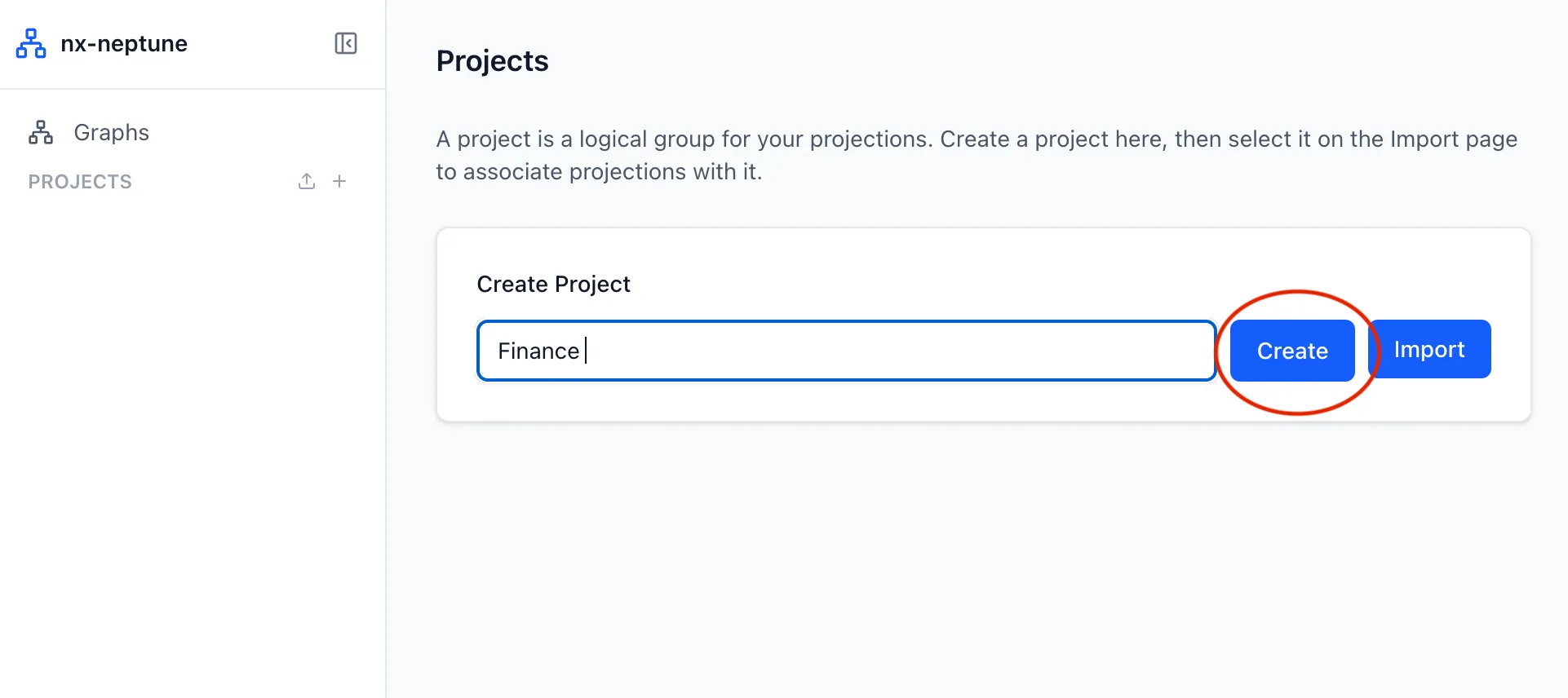
A project groups the graphs you build for one piece of work. In the sidebar, choose Add Project, enter a project name, and choose Create.
-
Add a graph
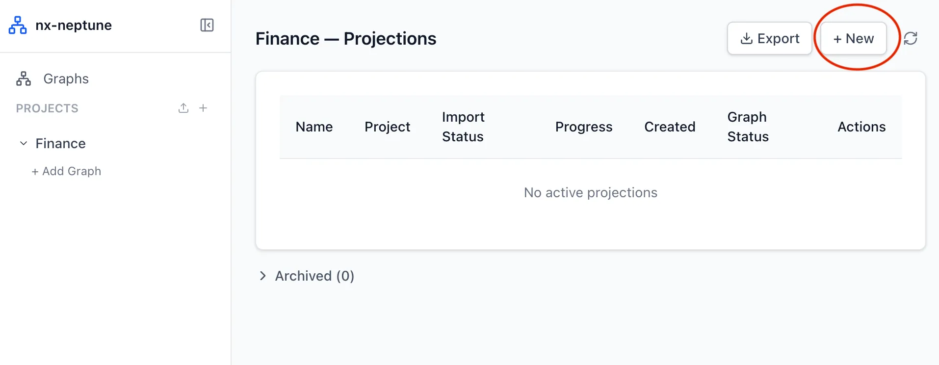
Under your project in the sidebar, choose + Add Graph. This opens the Import page for a new projection.
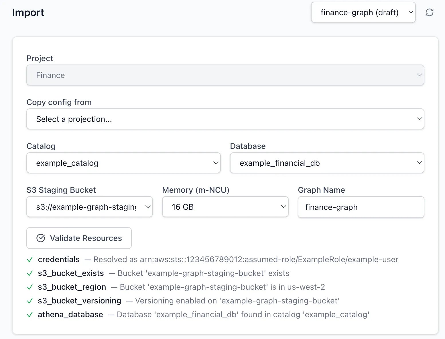
Choose the Athena Catalog and Database that contain your table, an S3 Staging Bucket for the exported data, the graph Memory (m-NCU), and a Graph Name. Choose Validate Resources to check that the proxy can reach them with your credentials.
-
Define the graph
Define the nodes and edges in one of two ways:
-
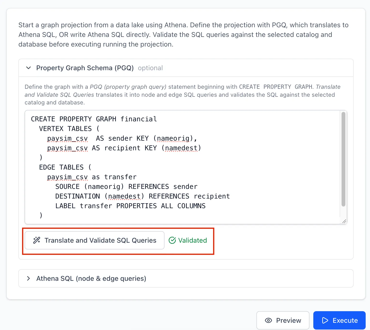
Property Graph Schema (PGQ): write a
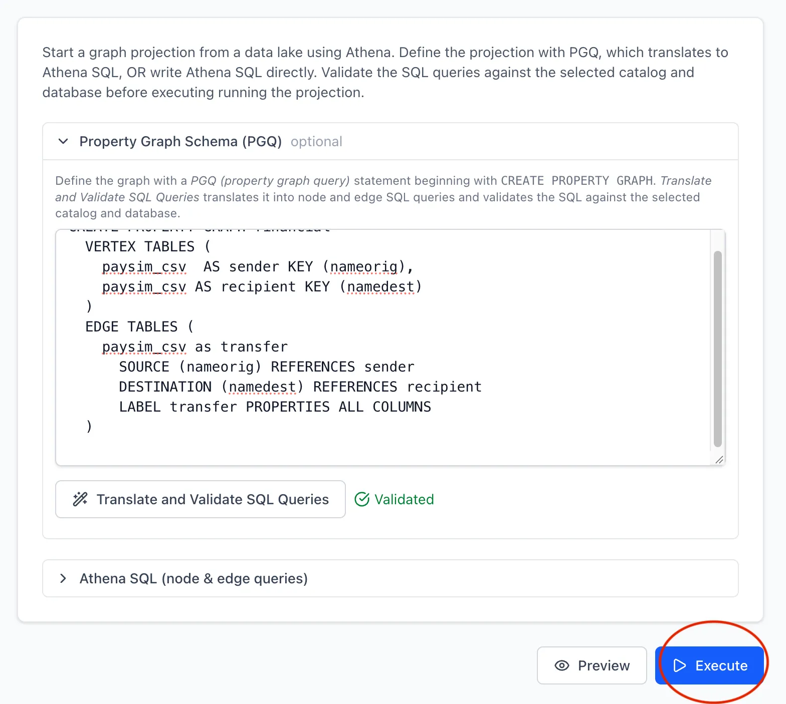
CREATE PROPERTY GRAPHstatement and choose Translate and Validate SQL Queries. The proxy translates it into node and edge queries and validates them against the selected catalog and database. See Property Graph Schema for the syntax.CREATE PROPERTY GRAPH financialVERTEX TABLES (paysim_csv AS sender KEY (nameorig),paysim_csv AS recipient KEY (namedest))EDGE TABLES (paysim_csv AS transferSOURCE (nameorig) REFERENCES senderDESTINATION (namedest) REFERENCES recipientLABEL transfer PROPERTIES ALL COLUMNS)Each vertex table gets its label from its alias (
senderandrecipient), and with noPROPERTIESclause it keeps all columns as properties.PROPERTIES ALL COLUMNSdoes the same for thetransferedges. -
Athena SQL (node & edge queries): write the node and edge queries yourself, using the Neptune load columns (
~idand~labelfor nodes;~from,~toand~labelfor edges), then choose Validate SQL Queries.
-
-
Preview the data
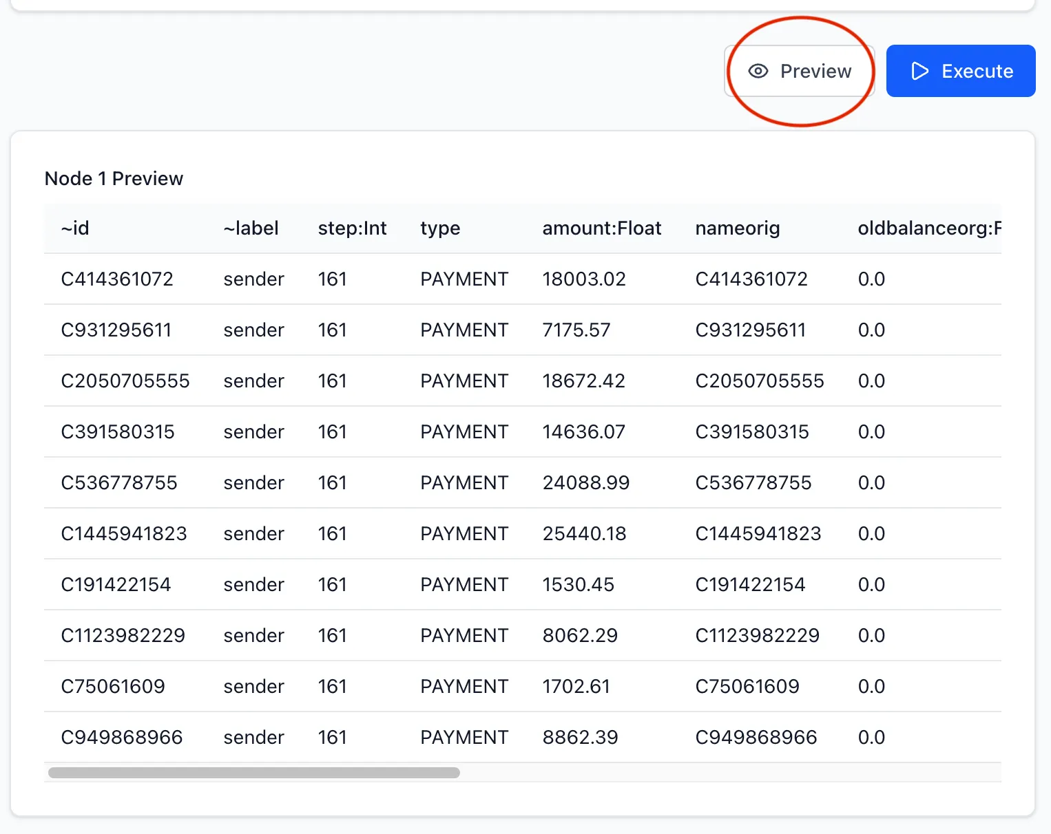
Choose Preview to see the first rows each node and edge query returns, and check that the ids, labels and properties look right before importing.
-
Run the import
Choose Execute. The proxy creates the Neptune Analytics graph, runs the queries in Athena, stages the results in S3, and imports them into the graph. Follow the Import Status and Progress columns on the projections page for your project. Creating the graph takes several minutes.
-
Check the graph
When the import completes, open Graphs in the sidebar to see the graph with its node and edge counts. The page shows the graphs that use the proxy’s name prefix (
nxp-by default). From here you can stop, start or delete the graph.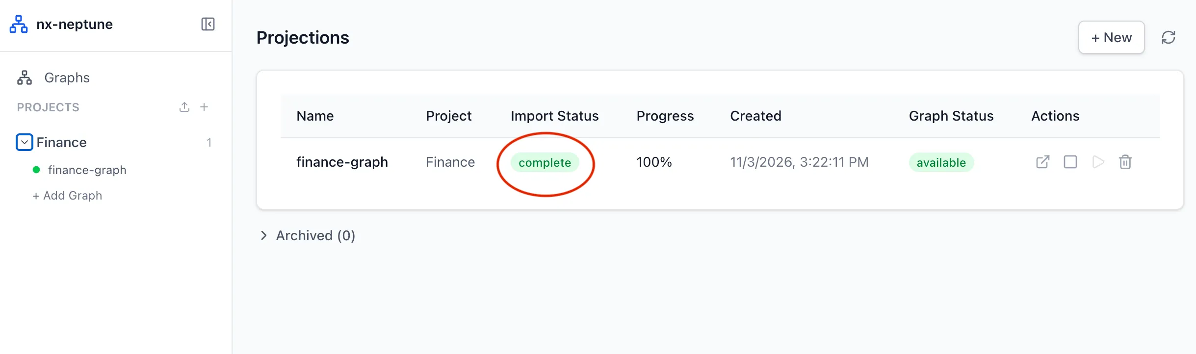
-
Open the graph in Graph Explorer
Start Graph Explorer if it isn’t running, as described in Start Graph Explorer.
Back in the proxy UI, choose Open in Graph Explorer on the graph. It’s available once the graph status is
AVAILABLE. Graph Explorer opens onhttps://localhost(or on the port you set withGE_PORT) with a connection to the graph filled in, using openCypher with IAM authentication. If the link shows a connection error, check that Graph Explorer is reachable withcurl -k https://localhost:<GE_PORT>/explorer/, and that its port isn’t used by another process.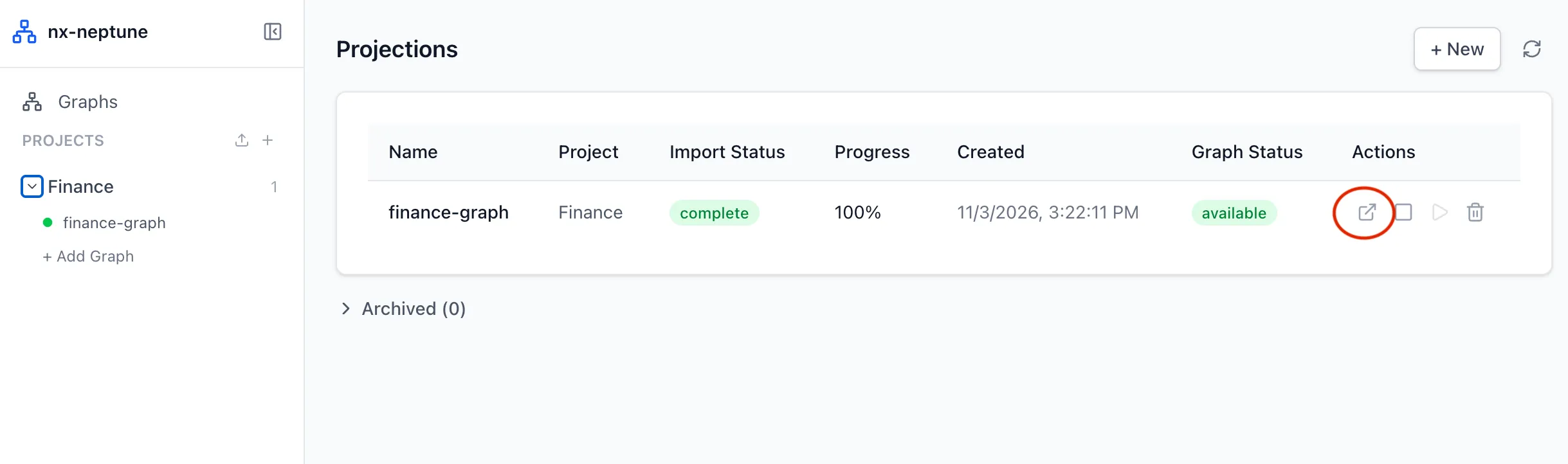
Run an openCypher query to explore the graph, for example the transfers marked as fraud:
MATCH (a:sender)-[t:transfer]->(b:recipient)WHERE t.isfraud = 1RETURN a, t, bLIMIT 50 -
Clean up
When you’re done, delete the graph so it stops incurring cost: choose Delete graph on the Graphs page, or Delete graph (archive projection) on the projections page, which keeps the projection’s configuration in the archived list. Then stop Graph Explorer with
make down.