Image Assets and Block-Level Access¶

The Simple Path¶

For straightforward reads — load an image, grab a region, pick specific bands — the convenience functions handle block assembly and asset selection for you:

from aws.osml.io import imread

# Full image as a NumPy array (bands, height, width)
pixels = imread("image.ntf")

# Windowed region — only reads the blocks that overlap
chip = imread("image.ntf", window=(100, 200, 256, 256))

# Select specific bands (zero-based)
rgb = imread("image.ntf", bands=[3, 2, 1])

# Reduced resolution (JPEG 2000 only)
thumbnail = imread("image.ntf", resolution_level=2)

When you need finer control — iterating individual blocks, checking for masked regions in sparse imagery, or working with the block grid directly — the block-level API described below gives you that access.

Tiled Images¶

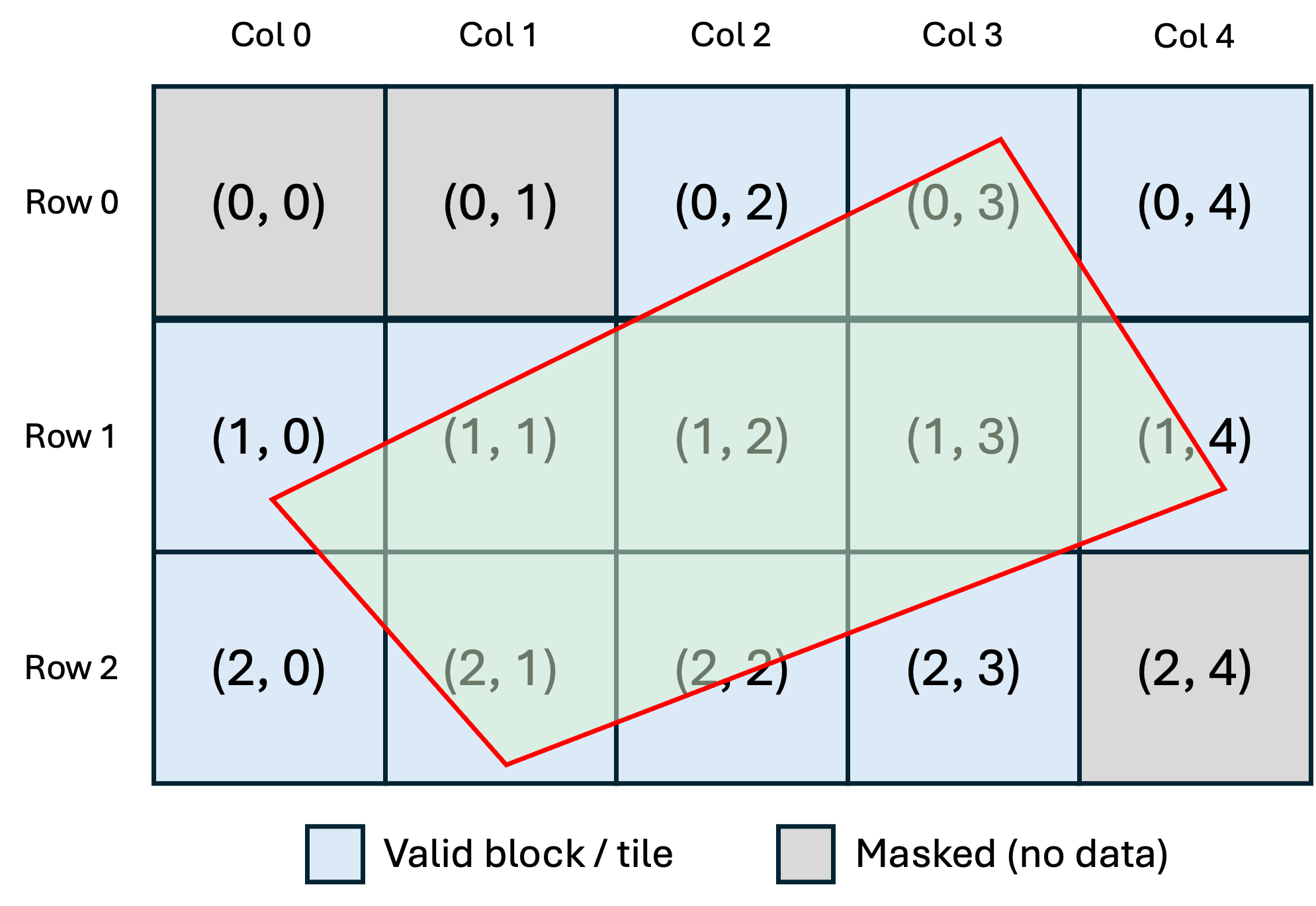
Large geospatial images are stored as tiled images. Rather than storing pixel data as one continuous stream, the image is divided into a regular grid of fixed-size rectangular regions called blocks (or tiles). Each block is addressed by its (row, col) position in the grid. This lets you read small regions efficiently without loading the entire image into memory.

Block grid diagram showing a 4x3 grid of blocks addressed by row and column, with two masked blocks

Both NITF and TIFF use this approach. In NITF, the image subheader defines the block dimensions (NPPBH × NPPBV) and the block grid size (NBPR × NBPC). In TIFF, the TileWidth and TileLength tags serve the same purpose. Stripped TIFFs are also supported — strips are treated as full-width blocks stacked vertically. When the image dimensions aren’t evenly divisible by the block size, edge blocks along the right and bottom boundaries may be smaller than the nominal block size.

from aws.osml.io import IO

with IO.open(["image.ntf"], "r") as dataset:
    image = dataset.get_asset("image:0")

    bands, height, width = image.image_shape
    _, block_h, block_w = image.block_shape
    grid_rows, grid_cols = image.block_grid_size

    print(f"Image: {width}x{height}, {bands} bands")
    print(f"Blocks: {block_w}x{block_h}, grid {grid_cols}x{grid_rows}")

Some formats, notably NITF, also support masked (sparse) images where not every position in the block grid contains data. The hatched cells in the diagram above represent masked blocks — regions with no pixel data. A block mask table in the file identifies which blocks are present, allowing empty blocks to be omitted entirely.

Iterating Over Blocks¶

get_block() always succeeds for valid grid coordinates. For masked (sparse) images, absent blocks return fill data — the pad pixel value from the mask table, or zero if none is defined. You can iterate over all blocks without guard checks:

grid_rows, grid_cols = image.block_grid_size

for row in range(grid_rows):
    for col in range(grid_cols):
        block = image.get_block(row, col, resolution_level=0)
        # Process block — filled with pad value if masked

Use has_block() to distinguish real image data from synthesized fill. This is useful when computing statistics, writing sparse outputs, or skipping unnecessary processing:

grid_rows, grid_cols = image.block_grid_size

valid = []
masked = []

for row in range(grid_rows):
    for col in range(grid_cols):
        if image.has_block(row, col, resolution_level=0):
            block = image.get_block(row, col, resolution_level=0)
            valid.append((row, col))
            # Process real image data...
        else:
            masked.append((row, col))

print(f"Valid: {len(valid)}, Masked: {len(masked)}")

Reading Blocks¶

get_block() returns a NumPy array with shape (bands, rows, cols). Geospatial images often carry more information than a simple RGB photograph. A panchromatic image has a single band of grayscale intensity. An RGB image has three bands (red, green, blue). Multispectral sensors capture additional bands beyond visible light — near-infrared (NIR), short-wave infrared (SWIR), and others — typically 3 to 10 bands, each covering a different wavelength range. Hyperspectral sensors push this further with hundreds of narrow contiguous bands spanning the electromagnetic spectrum. SAR (Synthetic Aperture Radar) imagery may store complex-valued data as separate magnitude/phase or in-phase/ quadrature (I/Q) band pairs.

The bands parameter lets you select which channels to decode. By default all bands are returned, but you can pass a list of zero-based band indices to retrieve only the ones you need. This is useful for extracting a natural-color composite from a multispectral image, isolating a single spectral band for analysis, or reading just the magnitude channel from a SAR product.

# All bands at full resolution
block = image.get_block(0, 0, resolution_level=0)

# Natural color from a multispectral image (bands 3, 2, 1 = R, G, B)
rgb = image.get_block(0, 0, resolution_level=0, bands=[3, 2, 1])

# Near-infrared band for vegetation analysis
nir = image.get_block(0, 0, resolution_level=0, bands=[4])

The resolution_level parameter controls the decode resolution. Some compression schemes, notably JPEG 2000, encode each block’s data at multiple resolution levels. This is a property of the compressed codestream within each block, not a separate set of overview images. The block grid stays the same — each block simply contains fewer pixels at higher level numbers.

Level	Scale	Example (2048×2048 block)
0	1:1	2048×2048
1	1:2	1024×1024
2	1:4	512×512
3	1:8	256×256

Uncompressed images and images using JPEG DCT compression have only one resolution level (level 0). Check available levels with image.num_resolution_levels.

# Iterate over all available resolution levels for a block
for level in range(image.num_resolution_levels):
    block = image.get_block(0, 0, resolution_level=level)
    bands, rows, cols = block.shape
    print(f"Level {level}: {cols}x{rows} ({bands} bands)")

Block-level resolution levels are different from overview assets. Overviews are separate images at reduced resolutions, exposed as distinct assets within the dataset. See Image Pyramids for how the library handles embedded overviews (COG) and multi-file pyramids (R-sets).

Known Limitations¶

JPEG 2000 Sub-Sampled Components¶

When a JPEG 2000 codestream contains components with non-uniform sub-sampling factors (XRsiz/YRsiz > 1, as in YCbCr 4:2:0 or 4:2:2 imagery), the library automatically upsamples all components to the reference grid using nearest-neighbor interpolation. The returned block always has uniform dimensions across all bands. This means sub-sampled components are spatially replicated — not interpolated with a reconstruction filter — which introduces blocky artifacts and does not preserve the native resolution of individual components. For scientific workflows that require access to components at their native sampling rate, this behavior is lossy and may not be acceptable.