Eigenmodes of a Cylindrical Cavity
The files for this example can be found in the examples/cavity/ directory of the Palace source code.
This example demonstrates Palace's eigenmode simulation type to solve for the lowest frequency modes of a cylindrical cavity resonator. In particular, we consider a cylindrical cavity filled with Teflon ($\varepsilon_r = 2.08$, $\tan\delta = 4\times 10^{-4}$), with radius $a = 2.74\text{ cm}$ and height $d = 2a$. From [1], the frequencies of the $\text{TE}_{nml}$ and $\text{TM}_{nml}$ modes are given by
\[\begin{aligned} f_{\text{TE},nml} &= \frac{1}{2\pi\sqrt{\mu\varepsilon}} \sqrt{\left(\frac{p'_{nm}}{a}\right)^2 + \left(\frac{l\pi}{d}\right)^2} \\ f_{\text{TM},nml} &= \frac{1}{2\pi\sqrt{\mu\varepsilon}} \sqrt{\left(\frac{p_{nm}}{a}\right)^2 + \left(\frac{l\pi}{d}\right)^2} \\ \end{aligned}\]
where $p_{nm}$ and $p'_{nm}$ denote the $m$-th root ($m\geq 1$) of the $n$-th order Bessel function ($n\geq 0$) of the first kind, $J_n$, and its derivative, $J'_n$, respectively.
In addition, we have analytic expressions for the unloaded quality factors due to dielectric loss, $Q_d$, and imperfectly conducting walls, $Q_c$. In particular,
\[Q_d = \frac{1}{\tan\delta}\]
and, for a surface resistance $R_s$,
\[Q_c = \frac{(ka)^3\eta ad}{4(p'_{nm})^2 R_s} \left[1-\left(\frac{n}{p'_{nm}}\right)^2\right] \left\{\frac{ad}{2} \left[1+\left(\frac{\beta an}{(p'_{nm})^2}\right)^2\right] + \left(\frac{\beta a^2}{p'_{nm}}\right)^2 \left(1-\frac{n^2}{(p'_{nm})^2}\right)\right\}^{-1}\]
where $k=\omega\sqrt{\mu\varepsilon}$, $\eta=\sqrt{\mu/\varepsilon}$, and $\beta=l\pi/d$.
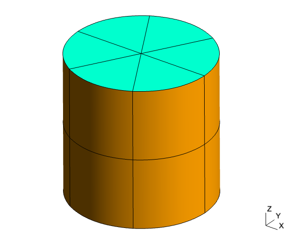
The initial Gmsh mesh for this problem, from mesh/cavity_prism.msh, is shown below. We use quadratic triangular prism elements. There are also two other included mesh files, mesh/cavity_tet.msh and mesh/cavity_hex.msh, which use curved tetrahedral and hexahedral elements, respectively.
There are two configuration files for this problem, cavity_pec.json and cavity_impedance.json.
In both, the config["Problem"]["Type"] field is set to "Eigenmode", and we use the mesh shown above. The material properties for Teflon are entered under config["Domains"]["Materials"]. The config["Domains"]["Postprocessing"]["Energy]" object is used to extract the quality factor due to bulk dielectric loss; in this problem since there is only one domain this is trivial, but in problems with multiple material domains this feature can be used to isolate the energy-participation ratio (EPR) and associated quality factor due to different domains in the model.
The only difference between the two configuration files is in the "Boundaries" object: cavity_pec.json prescribes a perfect electric conductor ("PEC") boundary condition to the cavity boundary surfaces, while cavity_impedance.json prescribes a surface impedance condition with the surface resistance $R_s = 0.0184\text{ }\Omega\text{/sq}$, for copper at $5\text{ GHz}$.
In both cases, we configure the eigenvalue solver to solve for the $15$ lowest frequency modes above $2.0\text{ GHz}$ (the dominant mode frequencies for both the $\text{TE}$ and $\text{TM}$ cases fall around $2.9\text{ GHz}$ frequency for this problem). A sparse direct solver is used for the solutions of the linear system resulting from the spatial discretization of the governing equations, using in this case a fourth-order finite element space.
The frequencies for the lowest-order $\text{TE}$ and $\text{TM}$ modes computed using the above formula for this problem are listed in the table below.
| $(n,m,l)$ | $f_{\text{TE}}$ | $f_{\text{TM}}$ |
|---|---|---|
| $(0,1,0)$ | –– | $2.903605\text{ GHz}$ |
| $(1,1,0)$ | –– | $4.626474\text{ GHz}$ |
| $(2,1,0)$ | –– | $6.200829\text{ GHz}$ |
| $(0,1,1)$ | $5.000140\text{ GHz}$ | $3.468149\text{ GHz}$ |
| $(1,1,1)$ | $2.922212\text{ GHz}$ | $5.000140\text{ GHz}$ |
| $(2,1,1)$ | $4.146842\text{ GHz}$ | $6.484398\text{ GHz}$ |
| $(0,1,2)$ | $5.982709\text{ GHz}$ | $4.776973\text{ GHz}$ |
| $(1,1,2)$ | $4.396673\text{ GHz}$ | $5.982709\text{ GHz}$ |
| $(2,1,2)$ | $5.290341\text{ GHz}$ | $7.269033\text{ GHz}$ |
First, we examine the output of the cavity_pec.json simulation. The file postpro/pec/eig.csv contains information about the computed eigenfrequencies and associated quality factors:
               m,             Re{f} (GHz),             Im{f} (GHz),                       Q
 1.000000000e+00,        +2.907188343e+00,        +5.814376364e-04,        +2.500000189e+03
 2.000000000e+00,        +2.924244826e+00,        +5.848489468e-04,        +2.500000129e+03
 3.000000000e+00,        +2.924244826e+00,        +5.848489421e-04,        +2.500000149e+03
 4.000000000e+00,        +3.471149740e+00,        +6.942299240e-04,        +2.500000137e+03
 5.000000000e+00,        +4.150836993e+00,        +8.301673534e-04,        +2.500000186e+03
 6.000000000e+00,        +4.150836993e+00,        +8.301673645e-04,        +2.500000153e+03
 7.000000000e+00,        +4.398026458e+00,        +8.796051788e-04,        +2.500000371e+03
 8.000000000e+00,        +4.398026459e+00,        +8.796053549e-04,        +2.499999871e+03
 9.000000000e+00,        +4.632147276e+00,        +9.264294365e-04,        +2.500000101e+03
 1.000000000e+01,        +4.632147278e+00,        +9.264294277e-04,        +2.500000125e+03
 1.100000000e+01,        +4.779153633e+00,        +9.558306713e-04,        +2.500000195e+03
 1.200000000e+01,        +5.005343455e+00,        +1.001068673e-03,        +2.500000096e+03
 1.300000000e+01,        +5.005389580e+00,        +1.001077846e-03,        +2.500000226e+03
 1.400000000e+01,        +5.005389580e+00,        +1.001077950e-03,        +2.499999965e+03
 1.500000000e+01,        +5.293474915e+00,        +1.058694964e-03,        +2.500000094e+03
Indeed we can find a correspondence between the analytic modes predicted and the solutions obtained by Palace. Since the only source of loss in the simulation is the nonzero dielectric loss tangent, we have $Q = Q_d = 1/0.0004 = 2.50\times 10^3$ in all cases.
Next, we run cavity_impedance.json, which adds the surface impedance boundary condition. Examining postpro/impedance/eig.csv we see that the mode frequencies are roughly unchanged but the quality factors have fallen due to the addition of imperfectly conducting walls to the model:
               m,             Re{f} (GHz),             Im{f} (GHz),                       Q
 1.000000000e+00,        +2.907188345e+00,        +7.091319575e-04,        +2.049821899e+03
 2.000000000e+00,        +2.924244827e+00,        +7.055966146e-04,        +2.072178956e+03
 3.000000000e+00,        +2.924244827e+00,        +7.055966604e-04,        +2.072178821e+03
 4.000000000e+00,        +3.471149742e+00,        +8.644493471e-04,        +2.007723102e+03
 5.000000000e+00,        +4.150836995e+00,        +9.792364835e-04,        +2.119425277e+03
 6.000000000e+00,        +4.150836995e+00,        +9.792365057e-04,        +2.119425229e+03
 7.000000000e+00,        +4.398026451e+00,        +1.000319808e-03,        +2.198310244e+03
 8.000000000e+00,        +4.398026457e+00,        +1.000319601e-03,        +2.198310702e+03
 9.000000000e+00,        +4.632147282e+00,        +1.054123330e-03,        +2.197156287e+03
 1.000000000e+01,        +4.632147282e+00,        +1.054125067e-03,        +2.197152665e+03
 1.100000000e+01,        +4.779153630e+00,        +1.126050842e-03,        +2.122086138e+03
 1.200000000e+01,        +5.005343456e+00,        +1.086214462e-03,        +2.304030995e+03
 1.300000000e+01,        +5.005389584e+00,        +1.171298237e-03,        +2.136684563e+03
 1.400000000e+01,        +5.005389585e+00,        +1.171297627e-03,        +2.136685675e+03
 1.500000000e+01,        +5.293474916e+00,        +1.207733736e-03,        +2.191490929e+03
However, the bulk dielectric loss postprocessing results, computed from the energies written to postpro/impedance/domain-E.csv, still give $Q_d = 1/0.004 = 2.50\times 10^3$ for every mode as expected.
Focusing on the $\text{TE}_{011}$ mode with $f_{\text{TE},010} = 5.00\text{ GHz}$, we can read the mode quality factor $Q = 2.30\times 10^3$. Subtracting out the contribution of dielectric losses, we have
\[Q_c = \left(\frac{1}{Q}-\frac{1}{Q_d}\right)^{-1} = 2.94\times 10^4\]
which is the same as the analytical result given in Example 6.4 from [1] for this geometry.
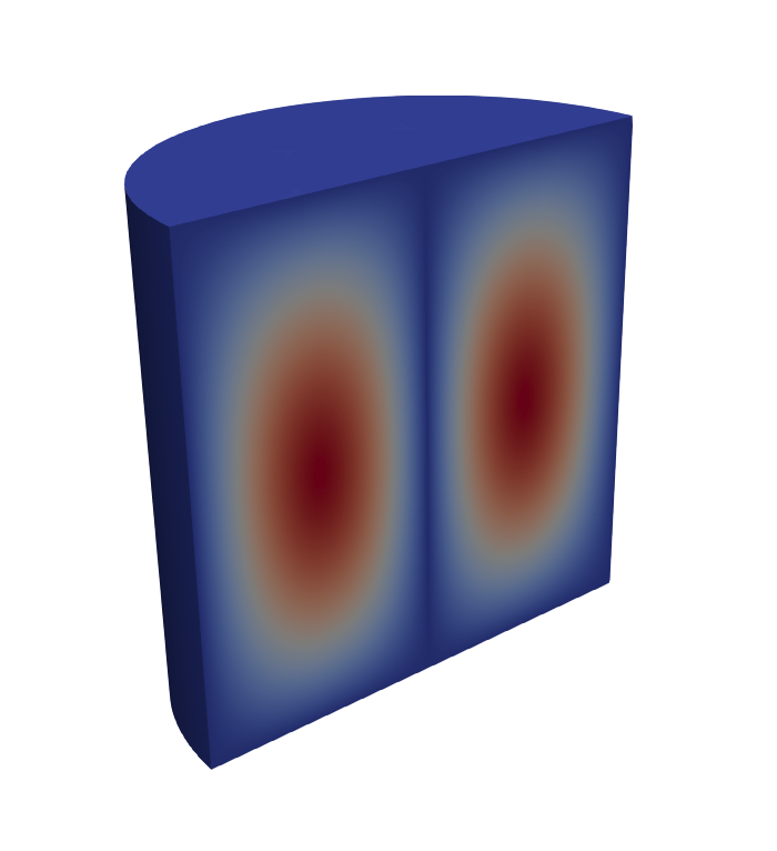
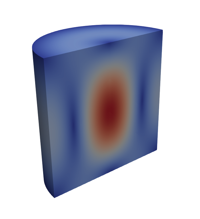
Finally, a clipped view of the electric field (left) and magnetic flux density magnitudes for the $\text{TE}_{011}$ mode is shown below.
Mesh convergence
The effect of mesh size can be investigated for the cylindrical cavity resonator using convergence_study.jl. For a polynomial order of solution and refinement level, a mesh is generated using Gmsh using polynomials of the same order to resolve the boundary geometry. The eigenvalue problem is then solved for $f_{\text{TM},010}$ and $f_{\text{TE},111}$, and the relative error, $\frac{f-f_{\text{true}}}{f_{\text{true}}}$, of each mode plotted against $\text{DOF}^{-\frac{1}{3}}$, a notional mesh size. Three different element types are considered: tetrahedra, prisms and hexahedra, and the results are plotted below. The $x$-axis is a notional measure of the overall cost of the solve, accounting for polynomial order.
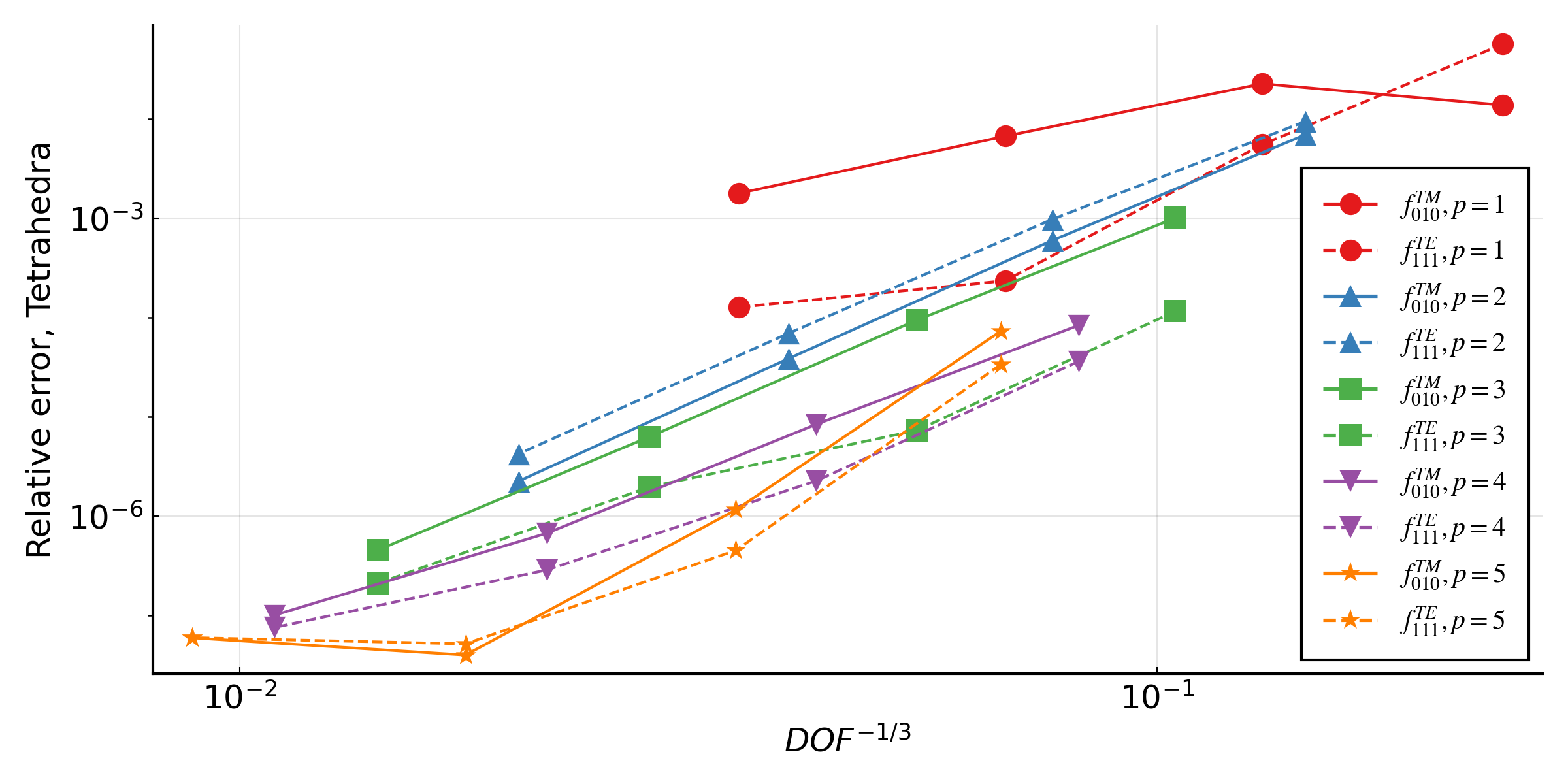
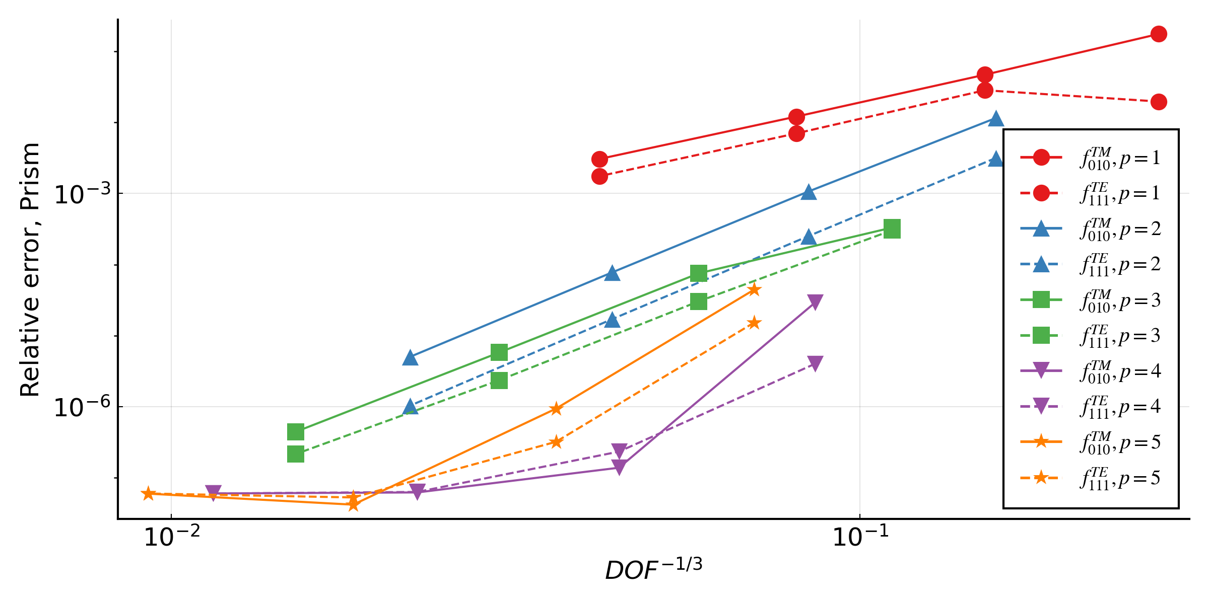
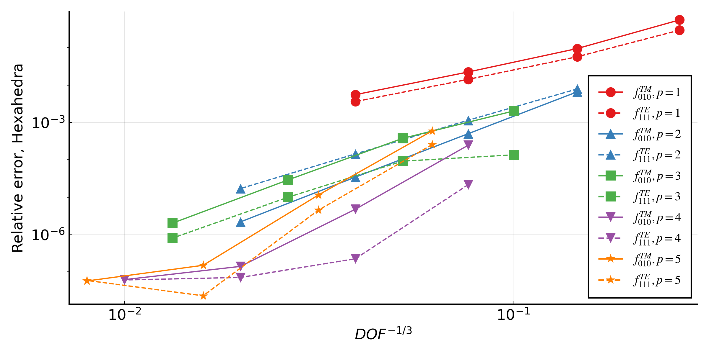
The observed rate of convergence for the eigenvalues are $p+1$ for odd polynomials and $p+2$ for even polynomials. Given the eigenmodes are analytic functions, the theoretical maximum convergence rate is $2p$ [2]. The figures demonstrate that increasing the polynomial order of the solution will give reduced error, however the effect may only become significant on sufficiently refined meshes.
References
[1] D. M. Pozar, Microwave Engineering, Wiley, Hoboken, NJ, 2012.
[2] A. Buffa, P. Houston, I. Perugia, Discontinuous Galerkin computation of the Maxwell eigenvalues on simplicial meshes, Journal of Computational and Applied Mathematics 204 (2007) 317-333.