Methods and citations
This page is for reviewers and for anyone who wants the math. It lists every statistical method the toolkit ships, the function that implements it, the formula, and the source it comes from. None of the statistics are new. The walkthrough explains each step in plain terms; this page is where the formulas live. Where the corrected-rate interval falls short of its stated coverage is on Reviewer notes.
Each step of the pipeline, and the published work it follows:
calibratecertifies a judge when the Wilson (1927) lower bounds on its TPR and TNR both clear the threshold, an intersection-union test (Berger 1982).run --judgecorrects the judge's flag rate (calibrated_agent_evaluation.calibrate.corrected_rate) with Rogan and Gladen (1978), the correction Lee et al. (2026) work out for LLM judges. The interval around it comes from Jeffreys posteriors (Brown, Cai and DasGupta 2001), not from Lee et al.'s construction.biaschecks the CALM biases of Ye et al. (2025), each bounded with Newcombe's (1998) paired interval.clusterreports saturation as Good–Turing coverage (Good 1953; Esty 1983) and Chao1 richness (Chao 1984, 1987).run --cigates each failure mode on a Wilson lower bound, again an intersection-union test.improvetests a fix with McNemar's (1947) paired test under Holm's (1979) correction.
Calibrated Agent Evaluation does not implement the hypothesis test of Feng et al. (2026) or the prediction-powered estimators studied by Chen et al. (2026) and packaged in GLIDE (Martinon, Merad and Raki 2026). Prior work says how each differs.
Methods by stage
| Stage | Method | Where it lives | Source |
|---|---|---|---|
calibrate |
Wilson score lower bound on TPR and TNR, one-sided 95% | calibrated_agent_evaluation.stats.wilson_lower, calibrated_agent_evaluation.calibrate.certify |
Wilson (1927) |
calibrate |
Certification as an intersection-union test over the two bounds | calibrated_agent_evaluation.calibrate.certify |
Berger (1982) |
calibrate |
Sample-size planner: the smallest per-class size from which the Wilson bound at the planned accuracy (correct count rounded down) clears the gate at every larger size, then the measured coverage floor | calibrated_agent_evaluation.calibrate.plan_calibration |
Wilson (1927); the coverage study below |
calibrate, run |
Minimum rate sample of 150 traces for a corrected rate | calibrated_agent_evaluation.calibrate.plan.MIN_RATE_SAMPLE |
the coverage study below; see Reviewer notes |
calibrate |
Youden's J, with the corrected point refused below 0.5 | calibrated_agent_evaluation.stats.rogan_gladen.youden_j |
Youden (1950) |
calibrate, run |
Rogan–Gladen prevalence correction | calibrated_agent_evaluation.stats.rogan_gladen.rogan_gladen |
Rogan and Gladen (1978) |
calibrate, run |
Corrected-rate interval from Jeffreys posteriors on TPR, 1 - TNR and the measured rate, with the modified Jeffreys rule at boundary counts | calibrated_agent_evaluation.stats.rogan_gladen.rg_interval |
Brown, Cai and DasGupta (2001) for the Jeffreys interval and its modification |
calibrate, run |
Design effect for verdicts clustered within a trace | calibrated_agent_evaluation.stats.rogan_gladen.cluster_design_effect |
Kish (1965); Korn and Graubard (1998) |
calibrate --explain |
Cohen's kappa with its large-sample interval and the confusion cells, for judge-versus-gold agreement on imbalanced gold (raw agreement with its Wilson interval otherwise) | calibrated_agent_evaluation.stats.kappa.cohen_kappa_interval, calibrated_agent_evaluation.enforce.display.agreement_display |
Cohen (1960); Fleiss, Cohen and Everitt (1969) |
bias |
Excess of each probe's disagreement rate over its placebo's, bounded by the one-sided 95% upper limit of Newcombe's paired interval, against a per-model threshold; for length and sycophancy, the same bound on directional moves toward the favored verdict over the placebo's, against 0.20; positional bias on pairwise judges only | calibrated_agent_evaluation.bias.run_battery |
Newcombe (1998); the CALM bias set of Ye et al. (2025) |
label, calibrate |
Krippendorff's alpha, Fleiss' kappa and per-class specific agreement, each with a unit-bootstrap interval; calibrate refuses gold from overlapping raters unless at least 130 traces are double-coded and alpha's lower bound reaches 0.80 |
calibrated_agent_evaluation.stats.agreement, calibrated_agent_evaluation.review.agreement |
Krippendorff (2004, 2011); Hayes and Krippendorff (2007); Fleiss (1971) |
cluster |
Good–Turing sample coverage with Esty's one-sided 95% lower bound | calibrated_agent_evaluation.cluster.saturation.good_turing_coverage_bound |
Good (1953); Esty (1983) |
cluster |
Chao1 richness with Chao's log-transformed 95% interval | calibrated_agent_evaluation.cluster.saturation.chao1_interval |
Chao (1984) for the estimator; Chao (1987) for the interval |
run |
CI gate: every mode's pass-rate Wilson lower bound must clear its threshold | calibrated_agent_evaluation.run.gate_mode_counts (the CLI's gate, over the verdicts in scope; calibrated_agent_evaluation.run.run_ci_gate is the library entry that also admits judges and scorers) |
Wilson (1927); Berger (1982) |
run --drift-baseline |
Benjamini–Yekutieli FDR at q = 0.10 over the two drift flags (PSI and Wasserstein) | calibrated_agent_evaluation.run.flag_slices, called by calibrated_agent_evaluation.run.drift_report.input_drift |
Benjamini and Yekutieli (2001) |
| library only | Benjamini–Yekutieli FDR at q = 0.10 over per-slice flags (a flag per taxonomy cell); calibrated-agent-evaluation run raises none until a per-slice test is specified |
calibrated_agent_evaluation.run.flag_slices |
Benjamini and Yekutieli (2001) |
run --drift-baseline |
Input drift on one --drift-feature: PSI on baseline-quantile bins and IQR-normalized Wasserstein distance, each with a permutation p-value, BY-FDR over the two; Jensen–Shannon divergence on the taxonomy-cell counts (the library default is the PSI bins) is reported but never flags |
calibrated_agent_evaluation.stats.drift, calibrated_agent_evaluation.run.drift_report.input_drift, calibrated_agent_evaluation.run.features |
Lin (1991) for JSD; Yurdakul and Naranjo (2020) for PSI |
run --drift-baseline |
Staleness warning for each judge admitted with --judge when input drift is flagged (a judge whose calibration no longer certifies it is not admitted, so it gets a "not admitted" note instead); never changes the gate, and --fail-on-drift gives it exit code 3 |
calibrated_agent_evaluation.run.check_staleness |
a rule over the drift flags above, no further statistic |
| library only | Judge drift: paired change in TPR or TNR with Newcombe's hybrid-score interval; no command computes it | calibrated_agent_evaluation.run.drift_report.judge_drift_paired, calibrated_agent_evaluation.stats.proportions.newcombe_paired_diff |
Newcombe (1998) |
calibrate --check, calibrate --explain |
Judge drift between two calibrations on independent gold: change in TPR or TNR with Newcombe's hybrid-score interval for independent proportions; the re-check's size is the smallest from which a judge showing 0.80 is flagged at every larger size | calibrated_agent_evaluation.run.judge_drift, calibrated_agent_evaluation.run.judge_check.check_size |
Newcombe (1998, independent proportions) |
plan --gate |
The gate's sample size: the smallest size from which the Wilson lower bound at the expected pass rate (count rounded down) clears the threshold at every larger size | calibrated_agent_evaluation.calibrate.gate_set_size |
Wilson (1927) |
improve |
McNemar's paired test: mid-p below 25 discordant pairs, uncorrected asymptotic above | calibrated_agent_evaluation.stats.mcnemar.mcnemar_paired |
McNemar (1947); Fagerland, Lydersen and Laake (2013) |
improve |
Holm correction over the guard panel at a family-wise alpha of 0.05 | calibrated_agent_evaluation.improve.panel.guard_panel |
Holm (1979) |
prefer |
Bradley–Terry ratings fitted by Hunter's MM iteration, 95% Wald intervals from the Fisher information under a sum-to-zero constraint; refused when the win graph is not strongly connected | calibrated_agent_evaluation.subjective.bradley_terry |
Bradley and Terry (1952); Hunter (2004); Ford (1957) |
probe |
pass^k over repeated trials, and an exact Clopper–Pearson interval on the per-trial rate | calibrated_agent_evaluation.probe.pass_hat_k, calibrated_agent_evaluation.probe.clopper_pearson |
Yao et al. (2024); Clopper and Pearson (1934) |
The Wasserstein distance is scipy.stats.wasserstein_distance divided by the pooled sample's
interquartile range. The project cites no primary source for it beyond the SciPy implementation.
A significant Wasserstein distance flags only above 0.10 (a tenth of the interquartile range),
so a negligible shift on a sample of thousands is not flagged. The null flag rate and the power at
four shift sizes are in fixtures/expected/drift/null_calibration.txt.
How the numbers work
A judge's raw rate
Take 1,000 production traces where 60 really failed (a true failure rate of 6%), and a judge that is right on 90% of failures and 90% of passes:
| Judge says FAIL | Judge says PASS | Total | |
|---|---|---|---|
| Trace really failed | 54 | 6 | 60 |
| Trace really passed | 94 | 846 | 940 |
| Total | 148 | 852 | 1,000 |
The judge reports 14.8%. The true-positive rate (TPR) is the share of real failures it flags, 54/60 = 0.90; the true-negative rate (TNR) is the share of real passes it leaves alone, 846/940 = 0.90. Both are properties of the judge and do not change with how common failures are. With true failure rate p, the share of traces flagged is
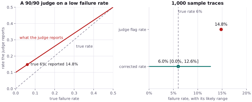
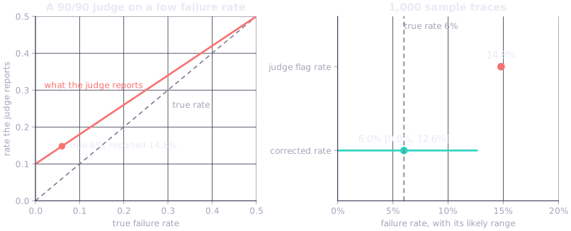
Certifying a judge
calibrate certifies a judge when the one-sided 95% Wilson score lower bounds on both its TPR and
its TNR reach 0.80 (fixed in code). Requiring both bounds is an intersection-union test (Berger 1982).
With k correct of n and z = 1.645:
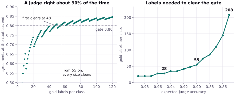
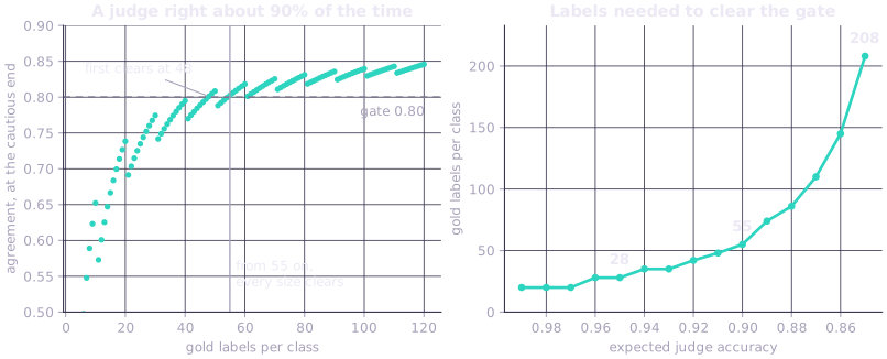
A judge about 90% right, by labels per class:
| Labels per class | Correct | Lower bound | Result |
|---|---|---|---|
| 20 | 18 | 0.738 | not certified |
| 35 | 32 (91.4%) | 0.804 | certified (31 correct, exactly 90%: 0.768, not certified) |
| 48 | 43 | 0.801 | exactly 90% first clears |
| 51 to 54 | 45 to 48 | 0.788 to 0.799 | the dip: not certified again |
| 55 | 49 | 0.803 | the plan: clears at every larger size too |
Because 90% of some sizes rounds down, the planner picks the smallest size from which every larger size clears:
about 90% observed accuracy, by labels per class:
  18/20 correct (90.0%): lower bound 0.738
  32/35 correct (91.4%): lower bound 0.804
  45/50 correct (90.0%): lower bound 0.808

labels per class to clear the 0.80 gate:
  expected accuracy 0.95: clears from  28 on, plan  80
  expected accuracy 0.90: clears from  55 on, plan  55
  expected accuracy 0.85: clears from 208 on, plan 208

the same judge, certified twice:
  18/20 per class: TPR lower bound 0.738, TNR lower bound 0.738: REFUSED
  32/35 per class: TPR lower bound 0.804, TNR lower bound 0.804: CERTIFIED
plan_calibration returns the larger of that size and the coverage floor (below):
plan_calibration(accuracy, 0.80) |
0.85 | 0.88 | 0.90 | 0.92 | 0.95 | 0.98 | 0.99 |
|---|---|---|---|---|---|---|---|
| To certify | 208 | 86 | 55 | 42 | 28 | 20 | 20 |
| The plan | 208 | 86 | 55 | 80 | 80 | 130 | 162 |
Judge-to-gold agreement is reported as TPR and TNR. calibrate --explain adds Cohen's kappa on
imbalanced gold.
Labels needed for a corrected rate
A judge can be certified to score and still not be trusted for a corrected rate. The range from the corrected rate needs a minimum number of gold labels per class, and that minimum depends on how accurate the judge turned out to be:
| Judge accuracy shown | 0.85 | 0.88 | 0.90 | 0.92 | 0.95 | 0.98 | 0.99 | up to 0.995 | 0.995 and up |
|---|---|---|---|---|---|---|---|---|---|
| Gold labels per class | 28 | 28 | 35 | 80 | 80 | 130 | 162 | 162 | 11 |
A more accurate judge needs more labels, because its range is built from its mistakes. A 98% judge on 50 labels makes about one mistake per class, and one mistake
is too little to estimate an error rate from. The gate checks the size at the accuracy you planned
for and again at the accuracy the judge showed, and the larger applies. A judge certified below this
size has a rate-unsafe record: it may still score, and calibrated-agent-evaluation run reports
its raw verdicts but refuses the corrected rate.
To be safe whatever accuracy the judge turns out to have, plan with --rate-safe
(rate_safe=True in the library). That asks for
162 per class at any planned accuracy from 0.88 to 0.99, and 208 at 0.85, where certification alone
needs more.
These sizes were measured by simulation, and a stronger rerun found that the range is still too narrow in a few cases they admit. Where the range falls short says where.
The corrected rate
The Rogan–Gladen correction (Rogan and Gladen 1978) runs the flagged-rate formula backwards:
The denominator, TPR + TNR - 1, is Youden's J (Youden 1950). Below J = 0.5 the corrected point is refused and the range is still reported. When the flag rate falls outside [1 - TNR, TPR] the point is not identifiable and is refused; the range is still reported.
TPR, the false-alarm rate 1 - TNR and the flag rate are each drawn from a Jeffreys posterior,
Beta(x + 1/2, n - x + 1/2) (Brown, Cai and DasGupta 2001), 9,999 draws, and the interval is the
middle 95% of the corrected values. At boundary counts (no errors on a class, or a rate sample with
no flags or all flags) the matching edge uses the modified Jeffreys rule from the same paper, which
only widens the interval. Span verdicts clustered within a trace are counted at their effective
size (Kish 1965).
from calibrated_agent_evaluation.stats.rogan_gladen import rg_interval, rogan_gladen

cal_pos = [1] * 154 + [0] * 8    # flagged 154 of 162 true FAILs: TPR 0.951
cal_neg = [1] * 8 + [0] * 154    # flagged 8 of 162 true PASSes: TNR 0.951
rate = [1] * 150 + [0] * 850     # flags 150 of 1,000 production traces: 15.0%

print(round(rogan_gladen(0.150, 154 / 162, 154 / 162), 4))
print(rg_interval(cal_pos, cal_neg, rate, seed=0))
0.1116
RGInterval(lo=0.06243283370392709, hi=0.14825398042693932, n_draws=9999, n_nonidentifiable=0, eval_design_effect=1.0)
The calibration set and the rate sample must be different traces: the calibration set is usually
hunted for failures, and only a random sample of traffic estimates production's rate. Passing the
calibration set as the rate sample raises SampleMisuseError, and the rate sample needs at least 150
traces.
Where the range falls short
The interval's coverage was measured by simulation (below). A rerun at 3,000 replicates per cell found two gaps. With 100 production traces at a 2% failure rate, coverage fell to about 92% for an accurate judge, which is why rate samples under 150 are refused. When a class of gold holds only two or three judge errors, the range is too narrow, with coverage as low as 91%; two such cases are inside what the gate allows (a 98% judge on 130 labels per class and a 99% judge on 260, both at failure rates of 5% or less with 100,000-trace rate samples). Failure rates below 2% were not simulated, and the simulation assumes judge errors are independent across traces. The cells, seeds and values are on Reviewer notes.
The bias check
Calibration shows a judge agrees with your labels on ordinary traces. It does not show whether the judge is swayed by things that should not matter. Before a certified judge may score, it runs a bias battery (based on the CALM set of biases in Ye et al. 2025): pairs of inputs that differ in one irrelevant way, such as a longer answer or a user insisting they are right. A judge that changes its verdict across the pair is showing that bias.
| Bias | Gates scoring? |
|---|---|
| length, self-preference, sycophancy | yes, must pass |
| distraction, bandwagon, compassion fade | no, recorded for you to read |
| positional | only for judges that compare two answers; skipped for single-verdict judges |
LLM judges are not perfectly consistent, so some verdicts flip even when nothing changed. To keep that from counting as bias, every trial comes with a placebo: the unchanged input judged again. The bias is how much more often the judge flips on the changed input than on the placebo. The check puts a 95% upper bound on that excess and compares it with a threshold set for the judge's model. A must-pass bias with no threshold configured refuses; no default is borrowed.
A worked number: in 12 trials, a judge flips its verdict 3 times when the answer is made longer and 0 times on the placebo. The excess is 3 in 12, 0.25, and its upper bound is 0.487. Against a threshold of 0.35 the judge is biased. Twelve trials is not many: a judge with no flips at all in 12 trials still has an upper bound of 0.184, so a threshold below that can never be met. Forty clean trials bring the bound down to 0.063.
The bound is Newcombe's interval for a paired difference (Newcombe 1998), since a trial and its placebo are judged on the same item. With no placebo flips it equals the Wilson upper bound on the trial flip rate.
Counting flips misses one case: a judge that is noisy on the plain answer but always passes the padded one flips about as often on the placebo as on the trial, so the excess looks like zero. Length and sycophancy probes therefore also say which verdict the change pushes toward (PASS for a padded answer, the asserted verdict for sycophancy). The check counts how often the changed input moves the verdict that way, compares it with how often the placebo makes the same move, and puts the same upper bound on the excess. That bound must stay under 0.20, set before the test was run on any judge. The quickstart's v1 judge fails it on both biases (sycophancy moved 2 of 12 trials toward the asserted verdict, none of the placebos did); v2 moves none of 30.
The CI gate
A mode passes when the one-sided 95% Wilson lower bound on its pass rate reaches the threshold (0.80
unless --threshold says otherwise). The gate reads the raw verdicts in scope from the source you
name: judge verdicts, code scorers or humans. Judge verdicts are gated only when every judge that made
them is admitted: its <judge_id>@<fingerprint> has a CERTIFIED calibration record and a CLEAR bias
battery in the store (with --judge FILE, the full admission chain runs on the file). The corrected rate is reported next to it and does not change the
exit code.
Nine passes in ten traces has a lower bound of 0.65, so it fails. A mode with no failures passes
from 11 traces; one that truly passes 90% of the time needs 55:
gate threshold: pass-rate 95% lower bound >= 0.80

failing traces in the mode   traces needed
   0                            11
   1                            20
   2                            28
   5                            48

true pass rate of the mode   traces needed
  1.00                          11
  0.97                          20
  0.95                          28
  0.90                          55
  0.85                         208
  0.80                        never passes
The build passes only when every gated mode passes. That is an intersection-union test (Berger 1982): each mode already gets through at most 5% of the time when it is truly bad, and requiring all of them can only make passing harder, so no multiple-comparison correction is needed.
Checking a fix
improve runs the same held-out inputs before and after the change and tests the discordant pairs
with McNemar's test (McNemar 1947): mid-p below 25 discordant pairs, the uncorrected asymptotic form
above, as Fagerland, Lydersen and Laake (2013) recommend. The size of the change gets Newcombe's
paired interval (Newcombe 1998). A fix is accepted when the two-sided test at 0.05 rejects in the
direction of a fall (in effect a one-sided test at 0.025), the whole interval clears the registered
minimum reduction, and no guard slice regressed under Holm's correction at a family-wise 0.05 (Holm
1979). The minimum reduction is registered before the after-run exists and frozen.
Saturation of failure modes
cluster estimates the probability that the next failure falls into a mode already seen with
Good–Turing coverage, 1 - (modes seen once / failures) (Good 1953), and Esty's one-sided 95% lower
bound (Esty 1983). On the bundled six-trace corpus, counting one observation per failing trace and
mode: 5 observations, 3 modes seen once, coverage 0.400, lower bound 0.000. Labeling is called saturated when the lower bound is at least 0.95, at least 30 failures are
labeled, and at least two modes were seen. Chao1 (Chao 1984) estimates the total number of modes,
with Chao's log-transformed interval (Chao 1987): 8.5 modes, between 4.5 and 44.9, on the same
corpus.
How many traces to double-code
Double-code the calibration gold itself: a second rater labels the same traces the judge will be calibrated on, so no extra traces are needed. The gate needs at least 130 traces labeled by both raters before it can say usable, because on a small overlap the interval says little: two raters who agree on all 20 shared traces get a lower bound of 1.0. Below 130 it answers "top up overlap", unless the high end of alpha's interval is already under 0.80 ("revise codebook") or under 0.667 ("codebook broken"). More shared traces narrow the interval but cannot lift it over a bar its high end is under. In 100 simulated sets of 60 shared traces from raters at alpha 0.30 (seed 20261027), 90 came out "codebook broken" and 10 "revise codebook"; raters at alpha 0.90 on 20 to 100 shared traces were never told to revise.
The 130 comes from the rule the label planner uses for the judge's gold. Plug in the agreement you
expect, alpha 0.90 on gold that is half PASS and half FAIL, round the counts against the raters,
and take the smallest overlap from which alpha's lower bound clears 0.80 there and at every larger
size (docs/site/examples/guides/overlap_size.py):
raters expected at alpha 0.9, 50% FAIL

shared traces   both FAIL / both PASS / split   lower bound   clears the gate
   50           23 / 24 / 3                     0.723         no
  100           47 / 48 / 5                     0.801         no
  110           52 / 52 / 6                     0.800         no
  122           57 / 58 / 7                     0.800         no
  130           61 / 62 / 7                     0.812         yes
  150           71 / 71 / 8                     0.814         yes
  200           95 / 95 / 10                    0.838         yes

minimum overlap: 130 (clears at every size from there to 1000)
The bound first clears at 100 and falls short again at 110 and 122, so the minimum is the size it
stays clear from. A size also needs a margin for the gate's own 2000 resamples, which move the
bound by about 0.007; that is why 100 shows "no" at 0.801. A gold planned at 55 traces per class is
110 traces, so double-coded gold is planned at 65 per class: calibrated-agent-evaluation calibrate --raters 2 plans
that, and so does calibrated-agent-evaluation calibrate on gold that already carries two raters' labels.
Raters who agree as planned clear the gate at 130 shared traces in most of their sets, not all: in
60 simulated sets of 130 traces from raters at alpha 0.90 (seed 7), 41 came out usable and the
rest were told to double-code more. calibrated_agent_evaluation.review.plan_overlap takes your own expected agreement
and FAIL rate.
Drift
run --drift-baseline compares one input feature between two random samples with PSI on ten
baseline-quantile bins (Yurdakul and Naranjo 2020) and the Wasserstein distance divided by the pooled
interquartile range, each with a permutation p-value, and Benjamini–Yekutieli FDR at q = 0.10 over the
two (Benjamini and Yekutieli 2001). A flag also needs the effect to clear its bar: 0.25 for PSI and
0.10 for the normalized Wasserstein distance. Jensen–Shannon divergence (Lin 1991) on the same bins
is reported and never flags. Fewer than 5 values per bin per side (50 with ten bins) is not measured.
On same-distribution splits the check flags 5.8% to 7.0% of the time; the null and power study is
fixtures/expected/drift/null_calibration.txt.
Ranking subjective qualities
prefer --rank fits Bradley–Terry ratings (Bradley and Terry 1952) by Hunter's MM iteration (Hunter
2004), with 95% Wald intervals from the Fisher information under a sum-to-zero constraint, shown on an
Elo-like scale where 400 points is 10:1 odds. When the win graph is not strongly connected (a trace
won or lost every comparison), the maximum-likelihood rating does not exist (Ford 1957) and the group
is refused. The sequential Elo that --explain prints is for display only.
Measured coverage of the corrected-rate interval
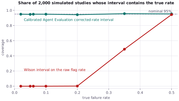
The corrected-rate interval's coverage was measured by Monte Carlo rather than assumed. The study
is calibrated_agent_evaluation.stats.studies.coverage, and its results are committed under
fixtures/expected/coverage/. tests/test_coverage_map.py re-measures named cells so the files
cannot drift from the shipped estimator.
| File | Cells | Replicates per cell | rg_interval coverage, lowest to highest |
Cells off 0.95 after Holm |
|---|---|---|---|---|
rg_interval_coverage.json (TPR = TNR) |
168 | 2000 | 0.932 to 0.962 | 0 of 168 |
rg_interval_coverage_asymmetric.json (TPR differs from TNR) |
840 | 2000 | 0.9295 to 0.965 | 0 of 840 |
The grid crosses expected judge accuracy 0.85 to 0.98, the per-class sizes the planner returns, prevalence 0.02 to 0.50, and rate-sample sizes 100 to 5000. A cell is off nominal when an exact binomial test of its covered count against 0.95 rejects after Holm across the file.
These figures come from 2,000 replicates per cell. A later rerun of the planner's floor grid at 3,000 replicates per cell found under-coverage where a class shows about two to three judge errors, including two configurations the shipped floor admits. Those cells, and the 150-trace rate-sample minimum they led to, are on Reviewer notes.
The same files record a naive Wilson interval on the uncorrected rate as a comparison arm. Its coverage of the true rate ranges from 0.0 to about 0.96 over the symmetric grid, because it estimates the judge's flag rate rather than the failure rate.
The planner's coverage floor (plan_calibration's coverage_floor) comes from a separate scan,
planner_floor_scan.json, summarized in planner_floor.json:
| Expected accuracy | 0.85 | 0.88 | 0.90 | 0.92 | 0.95 | 0.98 | 0.99 | 0.995 | 0.999 | 1.00 |
|---|---|---|---|---|---|---|---|---|---|---|
| Floor, per class | 28 | 28 | 35 | 80 | 80 | 130 | 162 | 11 | 11 | 11 |
The rows up to 0.99 were derived at 1,000 replicates per cell. The rows at 0.995, 0.999 and 1.0 were scanned at 3,000 replicates per cell with the boundary rule in place and pass on coverage at least nominal; an accuracy between 0.99 and 0.995 takes the larger floor, 162. Reviewer notes give their provenance.
Prior work on correcting LLM-judge rates
Correcting a judge-labeled rate with a small human-labeled sample was worked out for the LLM-judge case in 2026. This library implements a version of that correction and does not claim a new estimator.
- Lee et al. (2026) build intervals for the Rogan–Gladen-corrected judge rate that carry uncertainty from both the test set and the human-labeled calibration set, and add adaptive allocation of the calibration sample.
- Lang and Reiczigel (2014) derived confidence limits for prevalence adjusted for estimated sensitivity and specificity, the same problem in veterinary epidemiology.
- Feng et al. (2026) treat the question as a hypothesis test with finite-sample Type-I error control under calibration uncertainty. The gate here thresholds a Wilson bound instead and does not have that guarantee.
- Chen et al. (2026) characterize the conditions under which a prediction-powered estimator (Angelopoulos et al. 2023) has strictly smaller asymptotic variance than a measurement-error correction. The result is conditional. The Rogan–Gladen interval here is not variance-optimal, and the library ships no prediction-powered estimator.
- Martinon, Merad and Raki (2026) package prediction-powered estimators and samplers as a library, GLIDE.
- Dorner, Nastl and Hardt (2025) show that when the judge is no more accurate than the model under evaluation, no debiasing scheme halves the human labels required.
References
- Angelopoulos, A. N., Bates, S., Fannjiang, C., Jordan, M. I. and Zrnic, T. (2023). Prediction-powered inference. Science 382(6671):669–674. doi:10.1126/science.adi6000
- Benjamini, Y. and Yekutieli, D. (2001). The control of the false discovery rate in multiple testing under dependency. The Annals of Statistics 29(4):1165–1188. doi:10.1214/aos/1013699998
- Berger, R. L. (1982). Multiparameter hypothesis testing and acceptance sampling. Technometrics 24(4):295–300. doi:10.2307/1267823
- Bradley, R. A. and Terry, M. E. (1952). Rank analysis of incomplete block designs: I. The method of paired comparisons. Biometrika 39(3/4):324–345. doi:10.2307/2334029
- Brown, L. D., Cai, T. T. and DasGupta, A. (2001). Interval estimation for a binomial proportion. Statistical Science 16(2):101–133. doi:10.1214/ss/1009213286
- Chao, A. (1984). Nonparametric estimation of the number of classes in a population. Scandinavian Journal of Statistics 11(4):265–270.
- Chao, A. (1987). Estimating the population size for capture-recapture data with unequal catchability. Biometrics 43(4):783–791. doi:10.2307/2531532
- Chen, Y. T., Lu, S., Li, S., Guo, M. and Li, S. (2026). Efficient inference for noisy LLM-as-a-judge evaluation. arXiv:2601.05420.
- Clopper, C. J. and Pearson, E. S. (1934). The use of confidence or fiducial limits illustrated in the case of the binomial. Biometrika 26(4):404–413. doi:10.1093/biomet/26.4.404
- Cohen, J. (1960). A coefficient of agreement for nominal scales. Educational and Psychological Measurement 20(1):37–46. doi:10.1177/001316446002000104
- Dorner, F. E., Nastl, V. Y. and Hardt, M. (2025). Limits to scalable evaluation at the frontier: LLM as judge won't beat twice the data. ICLR 2025. arXiv:2410.13341.
- Esty, W. W. (1983). A normal limit law for a nonparametric estimator of the coverage of a random sample. The Annals of Statistics 11(3):905–912. doi:10.1214/aos/1176346256
- Fagerland, M. W., Lydersen, S. and Laake, P. (2013). The McNemar test for binary matched-pairs data: mid-p and asymptotic are better than exact conditional. BMC Medical Research Methodology 13:91. doi:10.1186/1471-2288-13-91
- Feng, C., Shen, M., Balashankar, A., Gerner-Beuerle, C. and Rodrigues, M. R. D. (2026). Noisy but valid: robust statistical evaluation of LLMs with imperfect judges. ICLR 2026. arXiv:2601.20913.
- Fleiss, J. L. (1971). Measuring nominal scale agreement among many raters. Psychological Bulletin 76(5):378–382. doi:10.1037/h0031619
- Fleiss, J. L., Cohen, J. and Everitt, B. S. (1969). Large sample standard errors of kappa and weighted kappa. Psychological Bulletin 72(5):323–327. doi:10.1037/h0028106
- Ford, L. R. Jr. (1957). Solution of a ranking problem from binary comparisons. The American Mathematical Monthly 64(8):28–33. doi:10.2307/2308513
- Good, I. J. (1953). The population frequencies of species and the estimation of population parameters. Biometrika 40(3–4):237–264. doi:10.1093/biomet/40.3-4.237
- Hayes, A. F. and Krippendorff, K. (2007). Answering the call for a standard reliability measure for coding data. Communication Methods and Measures 1(1):77–89. doi:10.1080/19312450709336664
- Holm, S. (1979). A simple sequentially rejective multiple test procedure. Scandinavian Journal of Statistics 6:65–70.
- Hunter, D. R. (2004). MM algorithms for generalized Bradley–Terry models. The Annals of Statistics 32(1):384–406. doi:10.1214/aos/1079120141
- Kish, L. (1965). Survey Sampling. Wiley.
- Korn, E. L. and Graubard, B. I. (1998). Confidence intervals for proportions with small expected number of positive counts estimated from survey data. Survey Methodology 24(2):193–201.
- Krippendorff, K. (2004). Content Analysis: An Introduction to Its Methodology, 2nd ed. Sage.
- Krippendorff, K. (2011). Computing Krippendorff's alpha-reliability. Annenberg School for Communication, University of Pennsylvania, departmental paper.
- Lang, Z. and Reiczigel, J. (2014). Confidence limits for prevalence of disease adjusted for estimated sensitivity and specificity. Preventive Veterinary Medicine 113(1):13–22. doi:10.1016/j.prevetmed.2013.09.015
- Lee, C., Zeng, T., Jeong, J., Sohn, J. and Lee, K. (2026). How to correctly report LLM-as-a-judge evaluations. ICML 2026. arXiv:2511.21140.
- Lin, J. (1991). Divergence measures based on the Shannon entropy. IEEE Transactions on Information Theory 37(1):145–151. doi:10.1109/18.61115
- Martinon, G., Merad, I. and Raki, M. (2026). Industrializing prediction-powered inference: the GLIDE library for reliable GenAI and agentic systems evaluation. ICML 2026 Workshop on Statistical Frameworks for Uncertainty in Agentic Systems. arXiv:2605.31278.
- McNemar, Q. (1947). Note on the sampling error of the difference between correlated proportions or percentages. Psychometrika 12(2):153–157. doi:10.1007/BF02295996
- Newcombe, R. G. (1998). Improved confidence intervals for the difference between binomial proportions based on paired data. Statistics in Medicine 17(22):2635–2650.
- Newcombe, R. G. (1998). Interval estimation for the difference between independent proportions: comparison of eleven methods. Statistics in Medicine 17(8):873–890.
- Rogan, W. J. and Gladen, B. (1978). Estimating prevalence from the results of a screening test. American Journal of Epidemiology 107(1):71–76.
- Wilson, E. B. (1927). Probable inference, the law of succession, and statistical inference. Journal of the American Statistical Association 22(158):209–212. doi:10.1080/01621459.1927.10502953
- Yao, S., Shinn, N., Razavi, P. and Narasimhan, K. (2024). τ-bench: a benchmark for tool-agent-user interaction in real-world domains. arXiv:2406.12045.
- Ye, J., Wang, Y., Huang, Y. et al. (2025). Justice or prejudice? Quantifying biases in LLM-as-a-judge. ICLR 2025. arXiv:2410.02736.
- Youden, W. J. (1950). Index for rating diagnostic tests. Cancer 3(1):32–35.
- Yurdakul, B. and Naranjo, J. (2020). Statistical properties of the population stability index. The Journal of Risk Model Validation. doi:10.21314/JRMV.2020.227