Image Warping & Orthorectification

Raw satellite and airborne imagery is acquired in the sensor’s native geometry — a coordinate system shaped by the platform’s orbit, the sensor’s viewing angle, and the terrain beneath. Pixels in this space do not map uniformly to positions on the ground. Two types of geometric displacement dominate:

• Perspective displacement — off-nadir viewing angles compress one side of the scene relative to the other, producing non-uniform ground sampling across the field of view.

• Relief displacement — elevated objects (buildings, hills) are shifted radially from the sensor’s sub-satellite point. A 30-story building viewed 30 degrees off-nadir can be displaced several pixels from its true ground footprint.

Orthorectification removes both effects by projecting pixels onto a map-accurate coordinate system using a sensor model and (optionally) a digital elevation model. The result is a north-up, scale-consistent image that can be overlaid on web maps, compared against other collects for change detection, or mosaicked with neighboring scenes without alignment artifacts.

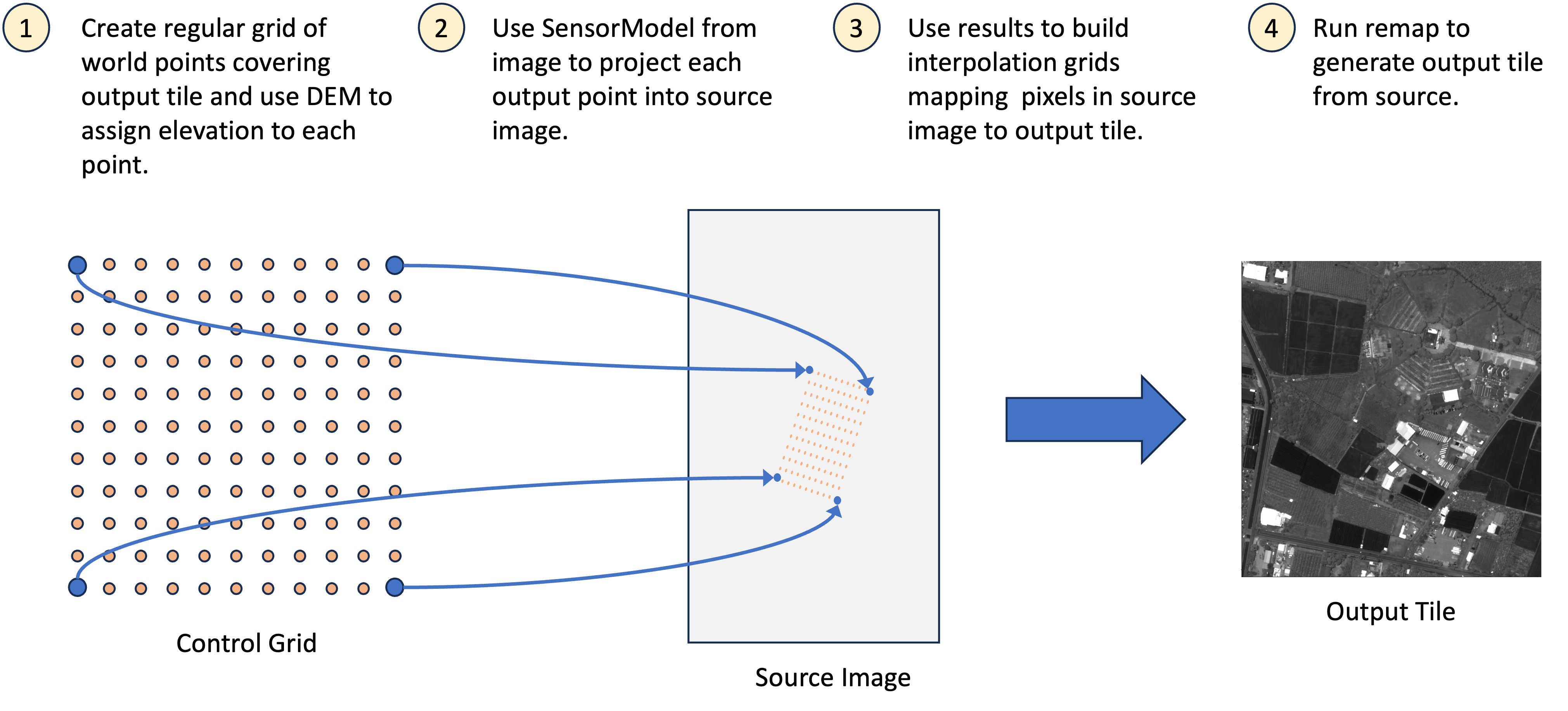
The toolkit’s warping engine uses the indirect method (also called reverse mapping): for each pixel in the output grid, it applies the inverse coordinate transformation to locate the corresponding position in the source image. This avoids the gaps that the direct method (source → output) would produce when output pixels fall between projected source samples. The inverse transformation may be a single sensor model, a chain of models (e.g. target image → world → source image), or any mapping that converts output coordinates to source coordinates.

Evaluating the full transformation at every output pixel is expensive, so the engine samples a sparse control grid at configurable density and interpolates the remaining positions via bilinear spline. A grid builder encapsulates this process — it defines the output coordinate system (map tiles, a projected CRS, or another image’s pixel space) and computes the control grid for each output block. The WarpedImageProvider then uses the grid builder to resample source pixels into the output geometry on demand.

Quick Start

Generate standard web map tiles from a georegistered image:

from aws.osml.io import IO
from aws.osml.metadata import load_sensor_model
from aws.osml.image_processing import (
    DisplayChainFactory,
    MapTileSetFactory,
    MappedImageProvider,
    OrthoGridBuilder,
    TiledImagePyramid,
    WarpedImageProvider,
    WarpGridOptions,
)

tile_set = MapTileSetFactory.get_for_id("WebMercatorQuad")

with IO.open("input.ntf", "r") as reader:
    source = reader.get_asset("image:0")
    sensor_model = load_sensor_model(reader)
    source_pyramid = TiledImagePyramid.from_dataset(reader)

    # Build a grid at zoom level 16
    grid_builder = OrthoGridBuilder(
        tile_set=tile_set,
        tile_matrix=16,
        sensor_model=sensor_model,
        source_width=source.num_columns,
        source_height=source.num_rows,
        options=WarpGridOptions.TERRAIN_CORRECTED,
        num_source_levels=source_pyramid.num_levels,
    )

    # Warp from the pyramid (reads at optimal resolution per block)
    warped = WarpedImageProvider(source_pyramid, grid_builder)

    # Apply display chain
    stats = source_pyramid.compute_statistics()
    chain = DisplayChainFactory.build(source, stats=stats)
    display = MappedImageProvider(
        warped, chain,
        source_bands=chain.input_bands,
        num_bands=chain.output_bands,
        pixel_value_type="uint8",
    )

    # Iterate tiles that overlap the source image
    min_row, min_col, max_row, max_col = grid_builder.tile_limits
    for tile_row in range(min_row, max_row + 1):
        for tile_col in range(min_col, max_col + 1):
            ortho_block = display.get_block(tile_row, tile_col)
            valid_mask = warped.get_valid_mask(tile_row, tile_col)
            # encode and write to z/x/y.png

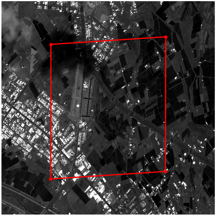
A map tile’s geographic boundary projected into source image coordinates. The non-rectangular polygon shows the sensor’s oblique viewing geometry.

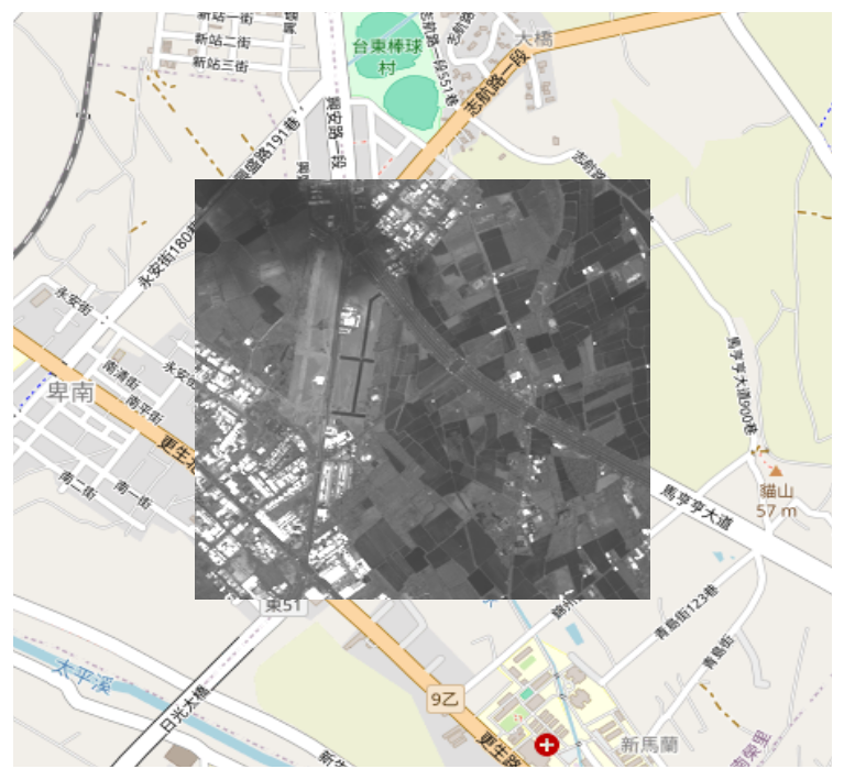
The resulting orthorectified tile overlaid on an OpenStreetMap background.

Reprojecting to a Map Grid

OrthoGridBuilder computes the inverse mapping from output tile pixels to source image coordinates. Pass a MapTileSet and tile matrix level, and it determines which tiles overlap the source image and how to warp each one.

Custom Projection (ProjectedImageTileSet)

For metric-unit output (meters/pixel) or any arbitrary CRS, use ProjectedImageTileSet to define a tile grid that covers the image footprint at a given GSD:

import pyproj
from aws.osml.image_processing import ProjectedImageTileSet

projected_tileset = ProjectedImageTileSet.from_sensor_model(
    sensor_model=sensor_model,
    source_width=source.num_columns,
    source_height=source.num_rows,
    target_crs=pyproj.CRS.from_epsg(32636),  # UTM Zone 36N
    gsd=0.5,  # 0.5 meters/pixel
    block_size=(1024, 1024),
)

grid_builder = OrthoGridBuilder(
    tile_set=projected_tileset,
    tile_matrix=0,  # level 0 = native GSD
    sensor_model=sensor_model,
    source_width=source.num_columns,
    source_height=source.num_rows,
    options=WarpGridOptions.TERRAIN_CORRECTED,
    num_source_levels=source_pyramid.num_levels,
)

warped = WarpedImageProvider(source_pyramid, grid_builder)

min_row, min_col, max_row, max_col = grid_builder.tile_limits
for r in range(min_row, max_row + 1):
    for c in range(min_col, max_col + 1):
        block = warped.get_block(r, c)

Any CRS supported by PROJ is valid — UTM, State Plane, Polar Stereographic, Web Mercator (EPSG:3857), etc. The gsd is in the CRS’s native units (meters for projected, degrees for geographic).

ProjectedImageTileSet also supports multi-resolution levels: level N covers 2^N x 2^N level-0 tiles at coarser resolution (same pixel dimensions per tile, larger geographic extent). Pass tile_matrix=1 for 2x overview, tile_matrix=2 for 4x, and so on.

With Elevation Model

For terrain-corrected output, provide an elevation model. Without one, the sensor model’s default elevation (typically the mean terrain height from image metadata) is used — adequate for flat terrain but insufficient for mountainous areas or urban scenes with tall buildings.

from aws.osml.elevation import ElevationModelBuilder, StoredDEMTileFactory
from aws.osml.photogrammetry import SRTMTileSet

elevation_model = (
    ElevationModelBuilder()
    .add_source(StoredDEMTileFactory("/path/to/srtm"), SRTMTileSet(format_extension=".dt2"))
    .add_fallback(0.0)
    .with_geoid("/path/to/egm96_15.tif")
    .build()
)

grid_builder = OrthoGridBuilder(
    tile_set=tile_set,
    tile_matrix=16,
    sensor_model=sensor_model,
    source_width=source.num_columns,
    source_height=source.num_rows,
    elevation_model=elevation_model,
    options=WarpGridOptions.TERRAIN_CORRECTED,
    num_source_levels=source_pyramid.num_levels,
)

See also

Elevation Models covers DEM source configuration, geoid correction, and multi-source fallback strategies in detail.

Co-Registering Two Images

When two images cover the same geographic area but were acquired at different times, from different orbits, or by different sensors, their pixel grids will not align. Change detection, temporal stacking, and multi-source fusion all require co-registering one image into another’s pixel space so that corresponding ground locations share the same (row, col) index.

ImageToImageGridBuilder produces this co-registration by chaining two sensor models: target image_to_world followed by source world_to_image. The result is a direct pixel-to-pixel mapping without an intermediate map projection step — preserving the target image’s native resolution and geometry:

from aws.osml.io import IO
from aws.osml.metadata import load_sensor_model
from aws.osml.image_processing import ImageToImageGridBuilder, WarpedImageProvider, WarpGridOptions

with IO.open("collect_2024.ntf", "r") as reader_a, \
     IO.open("collect_2025.ntf", "r") as reader_b:

    source_a = reader_a.get_asset("image:0")
    sm_a = load_sensor_model(reader_a)

    source_b = reader_b.get_asset("image:0")
    sm_b = load_sensor_model(reader_b)

    grid_builder = ImageToImageGridBuilder(
        source_sensor_model=sm_a,
        target_sensor_model=sm_b,
        source_width=source_a.num_columns,
        source_height=source_a.num_rows,
        target_width=source_b.num_columns,
        target_height=source_b.num_rows,
        block_width=source_b.num_pixels_per_block_horizontal,
        block_height=source_b.num_pixels_per_block_vertical,
        options=WarpGridOptions(control_points_per_side=16),
    )

    a_in_b = WarpedImageProvider(source_a, grid_builder)

    # Pixels are now co-registered — compare block-by-block
    for row in range(a_in_b.block_grid_size[0]):
        for col in range(a_in_b.block_grid_size[1]):
            block_a = a_in_b.get_block(row, col)
            block_b = source_b.get_block(row, col)
            # block_a and block_b are aligned — compute difference, etc.

Validity Masks

The warped output includes a per-block validity mask indicating which output pixels have actual source coverage:

warped = WarpedImageProvider(source, grid_builder)

block = warped.get_block(0, 0)       # CHW pixel data
mask = warped.get_valid_mask(0, 0)   # (H, W) bool array

# Use mask for alpha channel
alpha = (mask * 255).astype(np.uint8)

Invalid pixels are zero-filled. The mask is more reliable than checking for zero values, since legitimate source pixels may also be zero.

Control Grid Density & Performance

The control_points_per_side parameter controls the accuracy vs. speed tradeoff. Each control point requires a full sensor model evaluation (and optionally an elevation model lookup), so doubling the density quadruples the per-tile cost.

Preset	Control Points	Typical Use
WarpGridOptions.FAST	4x4 = 16	Real-time tile serving, previews
WarpGridOptions.TERRAIN_CORRECTED	16x16 = 256	Production ortho output
WarpGridOptions.VISIBILITY_AWARE	32x32 = 1024	High-fidelity (future)

Guidance:

• FAST (4x4) — Use for interactive map viewers, thumbnails, or any context where sub-pixel accuracy is unnecessary. Error stays below 1-2 pixels for typical RPC sensor models over flat terrain.

• TERRAIN_CORRECTED (16x16) — The default. Captures terrain undulation within a tile and produces sub-pixel accuracy for most production workflows. Required when an elevation model is supplied.

• Custom — Construct WarpGridOptions(control_points_per_side=N) for intermediate tradeoffs. Values of 8-12 work well for moderate terrain with RPC models; values above 16 yield diminishing returns unless the sensor model is highly nonlinear (e.g. RSM with many polynomial terms).

Factor	Impact	Mitigation
Sensor model complexity	RPC models are fast; RSM/SICD slower	Use FAST preset for interactive work
Control grid density	16x16 = 256 evaluations/block vs 4x4 = 16	Match density to accuracy requirements
Block size	Larger blocks amortize setup cost	Default 1024x1024 balances memory and throughput
Elevation model	First DEM tile load is slow; subsequent are cached	Pre-warm cache or use constant elevation for previews

Tip

For real-time tile serving, combine WarpGridOptions.FAST with a TileCache on the WarpedImageProvider to avoid recomputing grids for repeated requests to the same tile.

Related Topics

See also

• Tiling and Caching — TileCache and RetiledImageProvider used to normalize source layouts and cache decoded blocks

• Image Pyramids — how to build the source pyramid that enables resolution-aware warping

• Display Processing — the display chain applied to warped output for visualization

• Elevation Models — configuring terrain correction for accurate orthorectification